Robot Design|Bionic Ostrich Robot

It is National second prize winning works of the 10th National College Students Mechanical Innovation Design Competition.The funny thing is, it all started with an idea I had in the shower……
Prologue
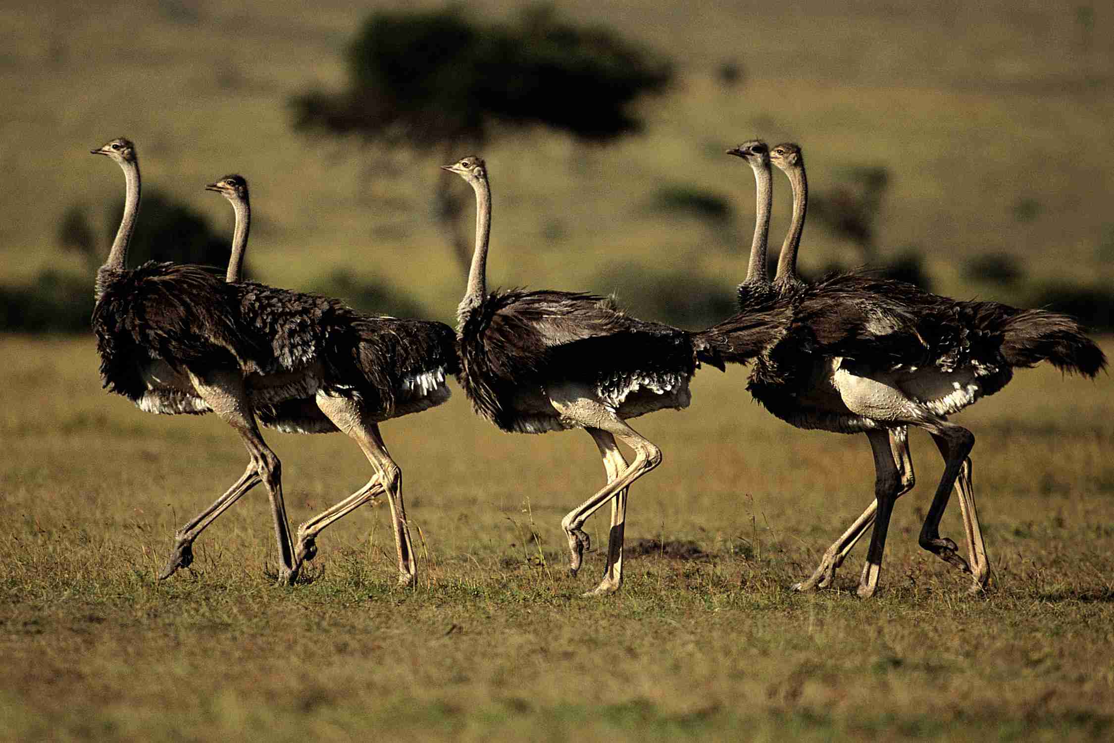
African ostriches
As the fastest running biped in the world, the ostrich has strong and powerful legs and can achieve continuous high-speed movement. This superiority provides an important reference value for the mechanical structure design of biped robots. Taking the ostrich leg as the bionic prototype, I designed a wheel-legged ostrich-like robot according to the principles of engineering bionics, and carried out relevant theoretical analysis and simulation experiment research.
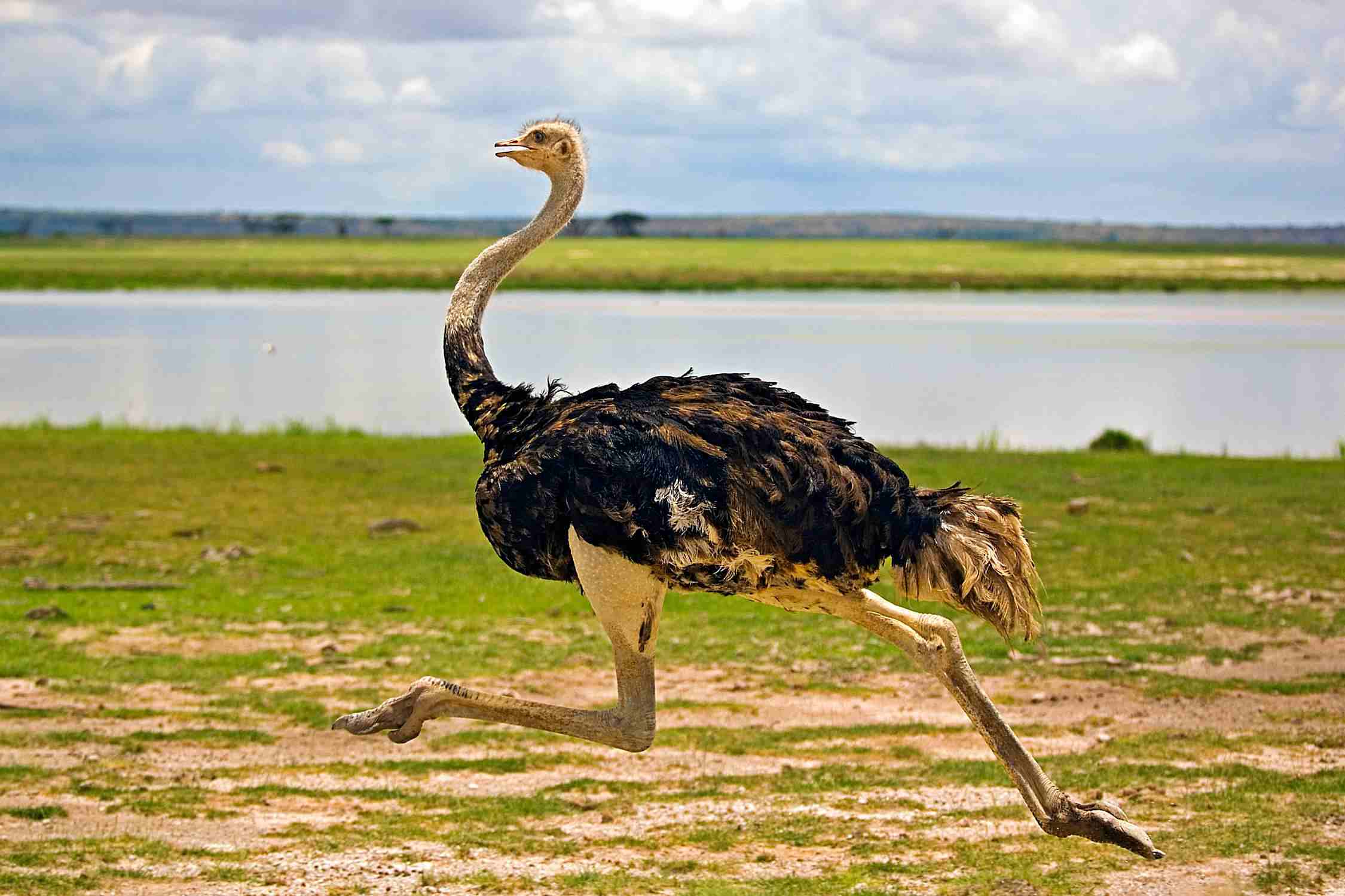
Running ostrich
In the process of designing an ostrich robot, I went through such steps:First of all, combined with the literature research method to study the biological mechanism, biological movement mechanism and movement law of ostriches, and summarize the reasons that make ostriches achieve continuous high-speed and stable running. Using bionic mechanical design and lightweight design, a wheel-legged ostrich-like robot with compact structure, simple control, high-speed running, energy saving and shock absorption is designed, and a 3D model is established through SOLIDWORKS. Secondly, the leg structure of the robot is simplified, and the forward kinematics mathematical model is established by vector analysis method, and the trajectory of the foot and the velocity and acceleration equations of each joint are obtained, and the correctness of the model is verified by ADAMS simulation. At the same time, the forward and inverse kinematics analysis of the leg mechanism of the robot is carried out, and its correctness is verified. Finally, based on D’Alembert’s principle, the dynamic analysis of the leg structure of the robot is carried out, a kinetostatics model is established, and the constraint reaction force of each joint and the driving torque required by the crank are solved, and the correctness of the dynamic model is verified by ADAMS simulation.
Design Background
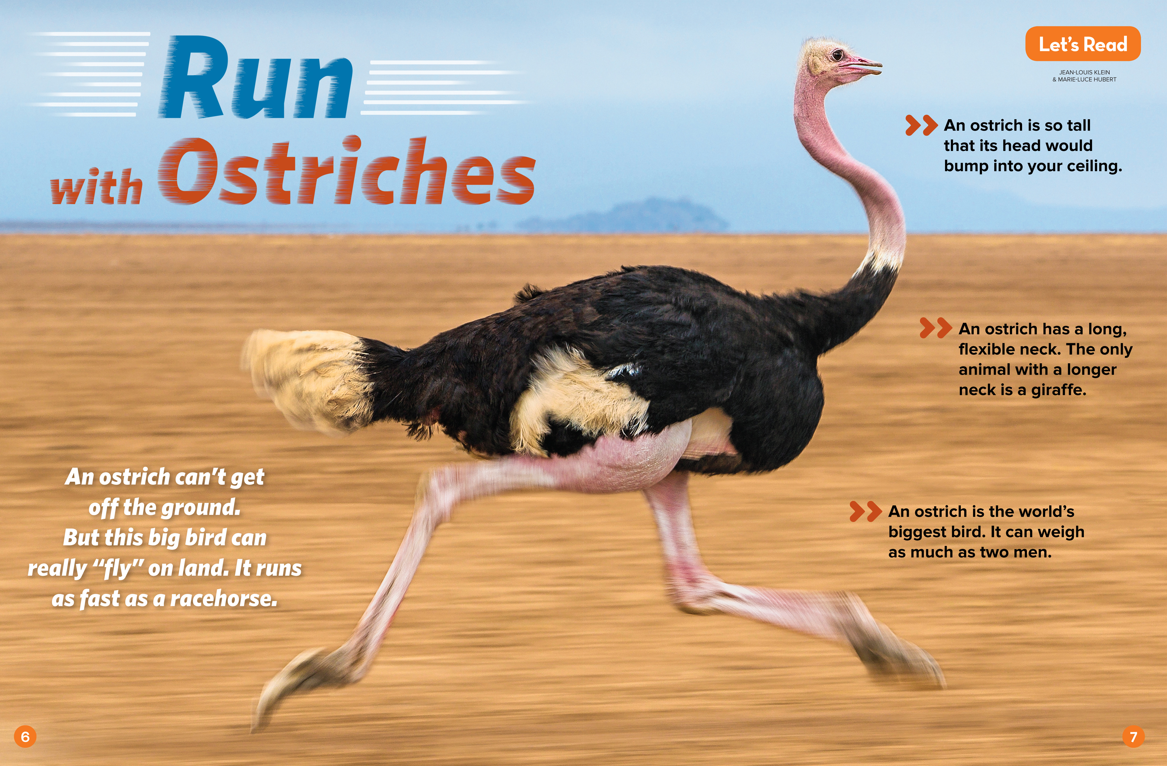
At present, the most bionic biped robots are humanoid biped robots. But the ostrich is one of the most efficient and durable large bipeds in existence. Ostrich legs have strong and powerful muscles, and under the interaction of leg bones-muscles-tendons, it has the characteristics of fast running speed, strong obstacle avoidance ability, stable and durable movement. The step length of each step of an ostrich during running can reach 3.5-7m, and it can run continuously at a speed of 50-60km/h for more than 30 minutes, and the fastest running speed can reach 70km/h. Compared with humans, the fastest running speed of ostriches is twice that of humans, and when the speed of movement exceeds 2km/h, the energy utilization efficiency of ostriches is about 1.5 times that of humans. Therefore, the ostrich provides important reference value in the research and bioinspired design of bioinspired biped robots with high energy efficiency and high speed.
Robot Design
Robot Design Metrics
The device should realize the basic function of bionic ostrich running. Mechanically capable of running fast. Remote control is possible on the control. And it is necessary to ensure that the device will not fall when it is running.
Structural Design
Analysis of biological characteristics of ostrich legs
The ostrich is the largest and heaviest biped animal in the world. It can run continuously for 30 minutes at an average speed of 50-60km/h. It is the fastest stable runner in the world, and its fastest running speed can reach 80km /h. According to the ostrich leg skeletal muscle model established by John R. Hutchinson et al., as shown in the figure, from top to bottom, the ostrich leg bones include femur, tibia, tarsal metatarsal, three phalanges and toenails, and the main joints include the hip joint , knee joint, ankle joint and metatarsophalangeal joint, the red line in the figure indicates the muscle-tendon structure of the ostrich leg. It can be seen from the figure that the ostrich legs have many double-joint or three-joint muscles connecting the knees, metatarsophalangeal joints, interphalangeal joints and toes, which can produce a high rigid-flexible coupling effect on the distal limbs of the ostrich, thereby coordinating the ostrich to complete Distal limb movement. In contrast, the hip joints of the ostrich legs are muscular, which mainly provide stability during the movement of the ostrich, and the joints directly used to adjust the posture of the ostrich limbs are the knee joints of the ostrich. The function of the ostrich knee joint is similar to that of the human hip joint, which can adjust the movement of the ostrich within a large range of motion.
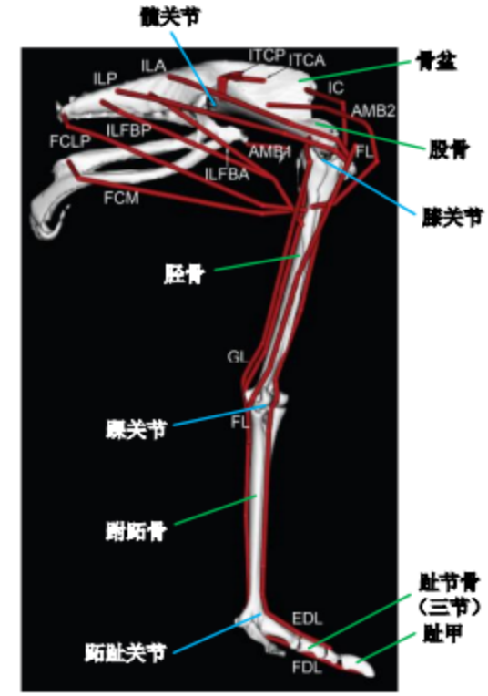
Illustration of ostrich leg skeletal muscle model
Therefore, the leg muscles of ostriches are mainly concentrated near the hip joints of ostriches, while the tibia and tarsal metatarsal bones are relatively light in mass, and are mainly driven by tendons or ligaments to generate movement, thereby reducing the mass of the distal end of the ostrich legs and reducing the rotation inertia. This facilitates the energy-efficient movement of the ostrich.
In order to enhance the output force of the muscles at the ostrich hip joint to the distal end of the leg, the rigid-flexible coupling leg of the ostrich combines the principle of leverage, so that the muscles and tendons are connected with the protruding part of the tibia at the knee joint of the ostrich and the contact of the tarsal metatarsal bone at the ankle joint. The protruding parts are connected to increase the acting moment by changing the effective limb length, and drive the ostrich legs to swing. The working principle is shown in figure below.
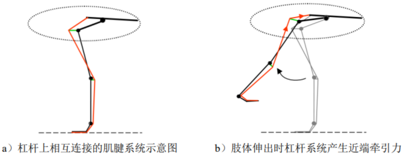
The principle of ostrich leg movement
In addition, the tendon acts as a buffer to delay when the muscle is exerted quickly and forcefully, thus effectively protecting the muscle from injury. The leg structure of the ostrich has well-developed tendon tissue. Through the rigid-flexible coupling characteristics of the tendon and the bone, the toe of the ostrich can partially convert the huge reaction force generated by the ground on its leg into the force of the bone before the toe touches the ground. The other part converts the impact energy into elastic potential energy and stores it by converting it into the tension of the tendon, and releases this energy at the end of the ground contact, thereby improving the movement efficiency of the ostrich. There is a passive rebound phenomenon in the joint between the ostrich tarsus and the tibia (ankle joint), which can be divided into three stages: first, the tibia is fixed, and then the joint angle between the tibia and the tarsus is changed by manipulating the tarsus; When the joint angle between the two bones is greater than 125°, the tarsus metatarsals will passively move to the maximum joint angle; when the joint angle between the two bones is less than 105°, the tarsus metatarsals will passively move to the minimum joint angle; when the joint angle between the two bones At the transition stage of 105°-125°, the passive rebound effect of this joint is not obvious, but when the joint angle between the two bones is 115°, the passive rebound phenomenon disappears, and the whole leg is in a balanced state. This passive rebound phenomenon can help the ostrich save energy consumption during exercise.
During the movement of an ostrich, when its toes are about to end touching the ground, under the action of tendons, the force at the toenails will change suddenly, causing the reaction force between it and the ground to suddenly increase, resulting in a “kicking force”. , to help the ostrich increase the speed of movement. In addition, the metatarsophalangeal joint of the ostrich is always off the ground, and there are tendons and ligaments in the metatarsophalangeal joint. By storing and releasing energy, it can buffer the impact of the ostrich when it moves at high speed, and can also save energy consumption.
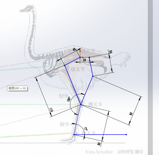
Among the ostrich leg bones, the femur near the trunk is short and thick, while the tibia and tarsus are relatively slender. According to the research of Nina U. Schaller, the average length of each bone in the ostrich leg and the total leg length are shown in table below, where the total leg length is equal to the sum of the lengths of all bones. It can be seen from this that the ratio of the lengths of the bones of the ostrich is:
$$ {14.70}:{30.65}:{30.65}:{34.95}:{34.95}:{19.70} $$
| femur length | tibial length | tarsal metatarsal length | third toe length | third toe length |
|---|---|---|---|---|
| 301.7 | 535.5 | 469.3 | 225.1 | 1531.4 |
Configuration selection
The main body of the leg of this device adopts a planar parallel five-bar mechanism, as shown in figure below, which consists of a main body and two bar groups. It imitates the morphological characteristics of ostrich legs in nature, and is a two-leg planar parallel mechanism. Compared with the series mechanism, the parallel mechanism has the characteristics of compact structure, high rigidity, and strong bearing capacity, which enables the robot to overcome obstacles more flexibly and move faster.
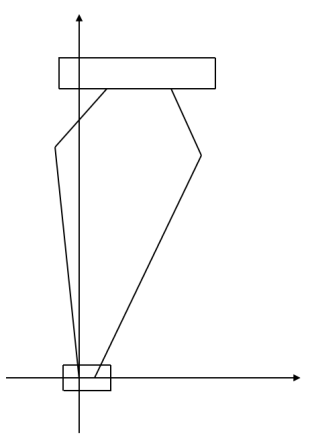
planar parallel five-bar mechanism
Each rotary joint of the main structure of the leg of the robot has two translation degrees of freedom along the transverse direction and the longitudinal direction respectively. Assuming that the robot moves in the x direction, it can be assumed to be symmetrical in the y (horizontal) direction. At the same time, the weight of the robot is mainly concentrated on the main structure and wheels.
The terminal structure of the device can be divided into two states of wheel type and step type, which can be transformed into each other through a special metamorphic mechanism during operation.
As shown in the figure below, the wheel rolls around the a-axis, thereby relying on the friction between the wheel and the ground to realize the forward and backward movement of the device as a whole.
As shown in the figure below, this device relies on the free rotation of the two hinge nodes at B and C to make the BC rod rotate rigidly. Adjust the angle between the BC rod and the ground by controlling the rotation degree at the two points B and C. The end prosthetic foot component and the BC rod are connected in a hinged manner. Due to its gravity, the connection line at the lowest point of the front and back palms is always parallel to the ground, which can be adaptively grounded.
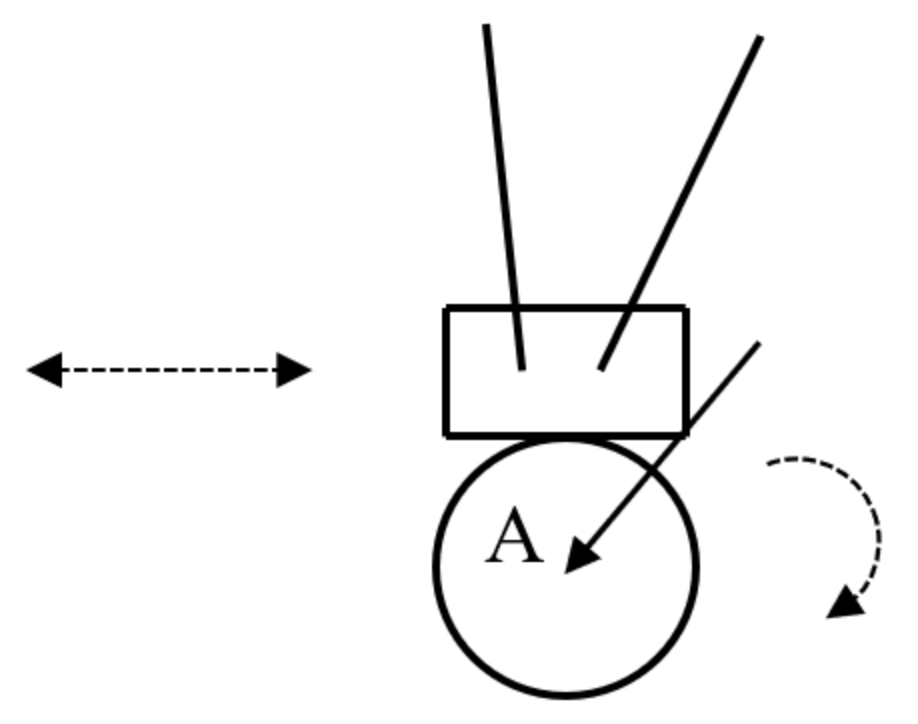
Wheel structure diagram
It should be noted that when standing, the BC rod is completely vertical, that is, the dead point of the connecting rod is on the same line, and the steering gear can stand firmly without outputting torque, which saves energy consumption.
As shown in the figure below, the BC rod continues to rotate counterclockwise until the foot member is completely off the ground and the wheel structure touches the ground, and then continues to rotate to nearly 90° with the ground. Because the mass of the forefoot in the foot component is greater than that of the backfoot, the center of gravity of the component is biased towards the forefoot. At this time, due to the effect of gravity, the foot member rotates clockwise around the hinge point C. And because of the clockwise rotation of the foot member, the BC bar continues to rotate counterclockwise, and the two form a positive feedback. And hinge B top has special device to hinder BC bar from continuing to rotate. When the BC bar rotates to this place, the structure is locked, and the foot is received by the top of the wheel and folded, thereby realizing the conversion of the wheel and foot. And the forefoot overlaps with the BC rod, which can prevent the contact between the foot and the ground from affecting the movement of the wheel.
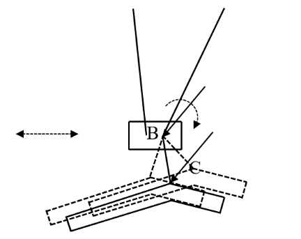
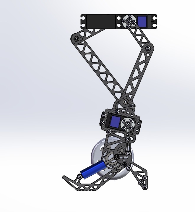
Leg structure diagram
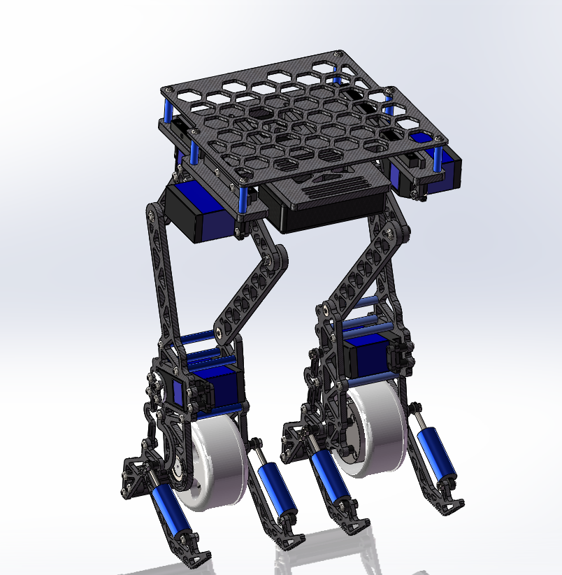
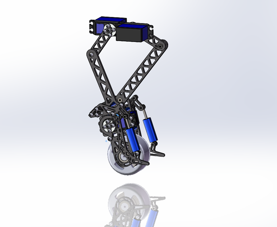
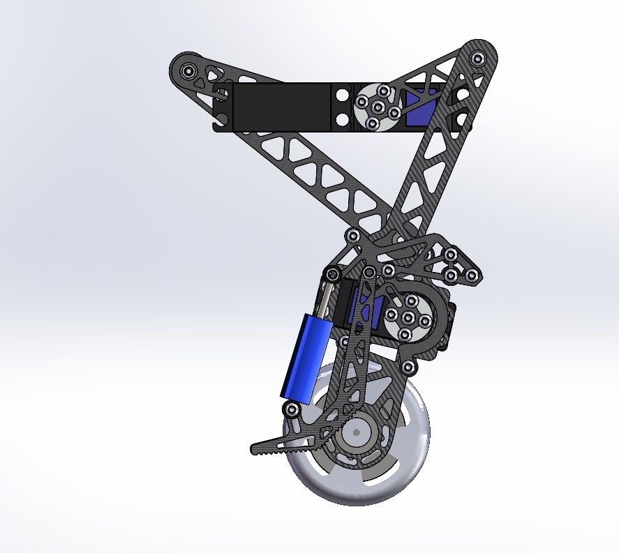
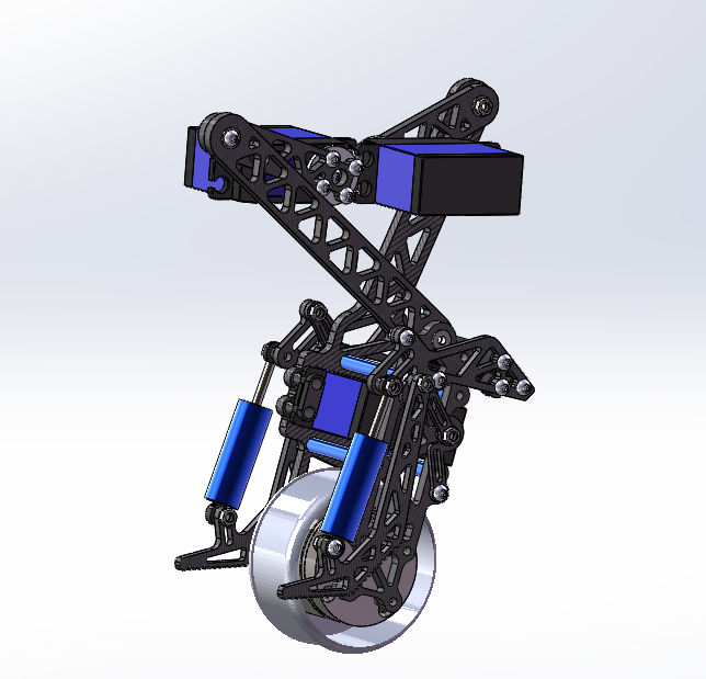
Overall picture of the robot
Mechanical Model Analysis
For the main structure of the legs, a simplified mathematical model of the closed-chain five-bar mechanism is established and placed on a plane Cartesian coordinate system, as shown in the left figure. The lengths of OA, CD, AB, BC, OD, and BE are $L_1$, $L_2$, $L_3$, $L_4$, $L_5$, and $L_6$, respectively. $O$ and $D$ points are driving. The overall structure can be regarded as an inverted pendulum structure, as shown in the right figure
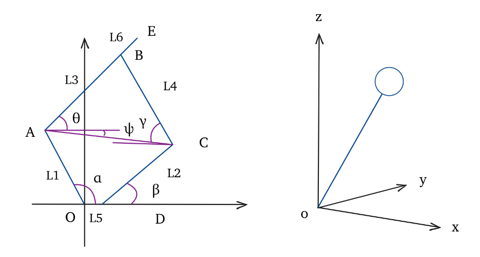
Simplified mathematical model schematic
Static analysis
- Closed chain five-bar mechanism
Forward kinematics solution:
We can know from the figure $$ \begin{aligned} \overrightarrow{O A}=\left(L_1 \cos \alpha, L_1 \sin \alpha\right)=\left(x_a, y_a\right) \end{aligned} $$
$$ \begin{aligned} \overrightarrow { OD }=\left(\begin{array}{ll} L 5,0 \end{array}\right) \end{aligned} $$
$$ \begin{aligned} \overrightarrow{D C}=\left(L_2 \cos \beta, L_2 \sin \beta\right) \end{aligned} $$
Due to $$ \begin{aligned} \overrightarrow{O C}=\overrightarrow{O D}+\overrightarrow{D C} \end{aligned} $$
So that $$ \begin{aligned} \overrightarrow{O C}=\left(L_5+L_2 \cos \beta, L_2 \sin \beta\right)=\left(x_c, y_c\right) \end{aligned} $$
Due to $$ \begin{aligned} \overrightarrow{A C}=\overrightarrow{O C}-\overrightarrow{O A} \end{aligned} $$
So that $$ \begin{aligned} |\overrightarrow{A C}|=\sqrt{\left(x_c-x_a\right)^2+\left(y_c-y_a\right)^2} \end{aligned} $$
From the law of cosines $$ \begin{aligned} \cos (\theta+\varphi)=\frac{\mathrm{L}_3{ }^2+|\overrightarrow{A C}|^2-L_4{ }^2}{2 L_3|\overrightarrow{A C}|} \end{aligned} $$
So that $$ \begin{aligned} \cos \theta \cos \varphi-\sin \theta \sin \varphi=\frac{L_3^2+|\overrightarrow{A C}|^2-L_4^2}{2 L_3|\overrightarrow{A C}|} \end{aligned} $$
Given that $$ \begin{aligned} \cos \varphi=\frac{x_c-x_a}{|\overrightarrow{A C}|} \end{aligned} $$
$$ \begin{aligned} \sin \varphi=-\frac{y_c-y_a}{|\overrightarrow{A C}|} \end{aligned} $$
So $$ \begin{aligned} 2 L_3\left(x_c-x_a\right) \cos \varphi+2 L_3\left(y_c-y_a\right) \sin \varphi=L_3^2+|\overrightarrow{A C}|^2-L_4^2 \end{aligned} $$
Let $$ \begin{aligned} A=2 L_3\left(x_c-x_a\right) \end{aligned}$$
$$ \begin{aligned} B=2 L_3\left(y_c-y_a\right) \end{aligned} $$
$$ \begin{aligned} C=L_3^2+|\overrightarrow{A C}|^2-L_4^2 \end{aligned} $$
So that $$ \begin{aligned} A \cos \varphi+B \sin \varphi=C \end{aligned} $$
Universal formula from trigonometric functions $$ \begin{aligned} \frac{A\left(1-\tan ^2 \frac{\theta}{2}\right)}{1+\tan ^2 \frac{\theta}{2}}+\frac{2 B \tan \frac{\theta}{2}}{1+\tan ^2 \frac{\theta}{2}}=C \end{aligned} $$
Solve the equation to get $$ \begin{aligned} \theta=2 \arctan \left(\frac{B \pm \sqrt{A^2+B^2-C^2}}{A+C}\right) \end{aligned} $$
Given that $$ \begin{aligned} \overrightarrow{A E}=\left(\left(L_3+L_6\right) \cos \theta\left(L_3+L_6\right) \sin \theta\right) \end{aligned} $$
$$ \begin{aligned} \overrightarrow{OE}=\overrightarrow{OA}+\overrightarrow{AE} \end{aligned} $$
We can know that $$ \begin{aligned} \overrightarrow{O E}=(x, y)=\left(x_a+\left(L_3+L_6\right) \cos \theta, y_a+\left(L_3+L_6\right) \sin \theta\right) \end{aligned} $$
Inverse kinematics solution:
We can know from the figure $$ \begin{aligned} \overrightarrow{O A}=\left(L_1 \cos \alpha, L_1 \sin \alpha\right) \end{aligned} $$
$$ \begin{aligned} \overrightarrow{O E}=(x, y) \end{aligned} $$
$$ \begin{aligned} \overrightarrow{A E}=\left(\left(L_3+L_6\right) \cos \theta\left(L_3+L_6\right) \sin \theta\right) \end{aligned} $$
Given that $$ \begin{aligned} \overrightarrow{O E}=\overrightarrow{O A}+\overrightarrow{A E} \end{aligned} $$
So that $$ \begin{aligned} \overrightarrow{O E}=(x \quad y)=\left(L_1 \cos \alpha+\left(L_3+L_6\right) \cos \theta L_1 \sin \alpha+\left(L_3+L_6\right) \sin \theta\right) \end{aligned} $$
Simplify to get $$ \begin{aligned} & 2 x L_1 \cos \alpha+2 y L_1 \sin \alpha=x^2+y^2+L_1^2-\left(L_3+L_6\right)^2 \end{aligned} $$
Let $$ \begin{aligned} & \mathrm{a}=2 \mathrm{xL}_1 \end{aligned} $$
$$ \begin{aligned} & \mathrm{~b}=2 \mathrm{yL}_1 \end{aligned} $$
$$ \begin{aligned} & c=x^2+y^2+L_1{ }^2-\left(L_3+L_6\right)^2 \end{aligned} $$
So $$ \begin{aligned} & a \cos \alpha+b \sin \alpha=c \end{aligned} $$
Solve the equation to get $$ \begin{aligned} & \alpha=2 \arctan \left(\frac{b \pm \sqrt{a^2+b^2-c^2}}{a+c}\right) \end{aligned} $$
Brought into the formula $$ \begin{aligned} & \overrightarrow{O E}=(x ,y)=\left(L_1 \cos \alpha+\left(L_3+L_6\right) \cos \theta L_7 \sin \alpha+\left(L_3+L_6\right) \sin \theta\right) \end{aligned} $$
Solve the equation to get $$ \begin{aligned} & \cos \theta=\frac{x-L_1 \cos \alpha}{L_3+L_6} \end{aligned} $$
$$ \begin{aligned} & \sin \theta=\frac{y-L_1 \sin \alpha}{L_3+L_6} \end{aligned} $$
So $$ \begin{aligned} & \overrightarrow{B E}=\left(L_6 \cos \theta, L_6 \sin \theta\right) \end{aligned} $$
Given that $$ \begin{aligned} & \overrightarrow{OB}=\overrightarrow{OE}+\overrightarrow{E B} \end{aligned} $$
We can know $$ \begin{aligned} \overrightarrow{OB}=(\mathrm{x}-\mathrm{L}_6 \cos \theta, \mathrm{y}-\mathrm{L}_6 \sin \theta)=(\mathrm{x}_b, \mathrm{y}_b) \end{aligned} $$
Given that $$ \begin{aligned} & \overrightarrow{O C}=\left(L_5 +L_2\cos \beta, L_2 \sin \beta\right) \end{aligned} $$
$$ \begin{aligned} & \overrightarrow{C B}=\left(-L_4 \cos \gamma, L_4 \sin \gamma\right) \end{aligned} $$
$$ \begin{aligned} & \overrightarrow{O B}=\overrightarrow{O C}+\overrightarrow{C B} \end{aligned} $$
We can know that $$\begin{aligned} & \mathrm{x}_{\mathrm{b}}=\mathrm{L}_5+\mathrm{L}_2 \cos \beta-\mathrm{L}_4 \cos \gamma \end{aligned}$$
$$\begin{aligned} & \mathrm{y}_{\mathrm{b}}=\mathrm{L}_2 \sin \beta+\mathrm{L}_4 \sin \gamma \end{aligned}$$
Eliminate $\gamma$ to get $$\begin{aligned} 2 L_2\left(x_b-L_5\right) \cos \beta+2 L_2 y_b \sin \beta=\left(x_b-L_5\right)^2+L_2{ }^2+y_b{ }^2-L_4{ }^2 \end{aligned}$$
Let $$\begin{aligned} d=2 L_2\left(x_b-L_5\right) \end{aligned}$$
$$\begin{aligned} e=2 L_2 y_b \end{aligned}$$
$$\begin{aligned} f=\left(x_b-L_5\right)^2+L_2{ }^2+y_b{ }^2-L_4{ }^2 \end{aligned}$$
So that $$\begin{aligned} d \cos \beta+e \sin \beta=f \end{aligned}$$
Solve the equation to get $$\begin{aligned} \beta=2 \arctan \left(\frac{e \pm \sqrt{d^2+e^2-f^2}}{d+f}\right) \end{aligned}$$
In summary $$\begin{aligned} \alpha=2 \arctan \left(\frac{b \pm \sqrt{a^2+b^2-c^2}}{a+c}\right) \end{aligned}$$
$$\begin{aligned} \beta=2 \arctan \left(\frac{\left.e \pm \sqrt{d^2+e^2-f^2}\right)}{d+f}\right) \end{aligned}$$
Therefore, the constraint reaction force of the force acting at E (set as F) on the robot leg end (O and D) can be expressed as
$$\begin{aligned} M_O=\left(\left(\mathrm{L}_3+\mathrm{L}_6\right) \cos \theta+\mathrm{L}_1 \cos \alpha\right) F \end{aligned}$$
$$\begin{aligned} M_D=\left(\left(\mathrm{L}_3+\mathrm{L}_6\right) \cos \theta+\mathrm{L}_1 \cos \alpha-\mathrm{L}_5\right) F \end{aligned}$$
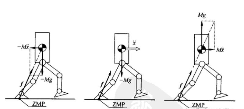
- Inverted pendulum mechanism
Consider a three-dimensional linear inverted pendulum model moving in three-dimensional Cartesian space, which rotates around point $O$, and the center of mass can move within a virtual constrained planar motion. The plane where $xy$ is located is the horizontal ground, the z-axis is vertical upwards, and is perpendicular to the ground, and we specify the positive direction of $x$ as the forward direction of the robot.
The constraint plane can be expressed using the normal vector of the plane as
$$\begin{aligned} \left(k_x, k_y-1\right) \end{aligned}$$
and the intersection of the z-axis with this plane is $Z_c$. Then for the constraint plane: $$\begin{aligned} z=k_x x+k_y y+z_c \end{aligned}$$
If the constraint plane is horizontal, then one has $$\begin{aligned} k_x=k_y=0 \end{aligned}$$
Even for the slope walking process where the constraint plane is not horizontal, we can add additional constraints to the torque to make the dynamic process hold: $$\begin{aligned} \tau_x x+\tau_y y=0 \end{aligned}$$
For the case where the constraint plane is horizontal, the zero moment point (ZMP) is calculated as $$\begin{aligned} p_x=-\frac{\tau_y}{m g} \end{aligned}$$
$$\begin{aligned} p_y=\frac{\tau_x}{m g} \end{aligned}$$
Kinematic analysis
The robot is composed of a main body and two legs with driving wheels as the ends. It imitates the morphological characteristics of ostrich legs in nature, and is a two-leg planar parallel mechanism. Compared with the series mechanism, the parallel mechanism has the characteristics of compact structure, high rigidity, and strong bearing capacity. As a result, the robot can run faster while overcoming obstacles with greater agility. At the same time, the device has two states of wheel type and step type, which can be transformed into each other during operation.
The robot is composed of a main body and two legs with driving wheels as the ends. It imitates the morphological characteristics of ostrich legs in nature, and is a two-leg planar parallel mechanism. Compared with the series mechanism, each rotary joint on the parallel robot leg has two translation degrees of freedom along the transverse direction and the longitudinal direction respectively. When the robot is running along the $x$ direction, it can be assumed to be symmetric in the $y$ (lateral) direction. At the same time, the weight of the robot is mainly concentrated on the main structure and wheels. Therefore, the robot can be approximated as an inverted pendulum on an industrial computer (IPC), and its dynamic equation is
$$ \begin{aligned} (\mathrm{M}+\mathrm{m}) \ddot{\mathrm{x}}+\mathrm{ml} \cos (\theta) \ddot{\theta}-\mathrm{ml} \sin (\theta) \dot{\theta}^2=\mathrm{u} \end{aligned}$$
$$\begin{aligned} \mathrm{ml} \cos \ddot{\mathrm{x}}+\mathrm{ml}^2 \ddot{\theta}-\mathrm{mgl} \sin (\theta)=0 \end{aligned}$$
Among them, $M$ and $m$ are the point mass concentrated at the tip of the pole and the mass of the trolley, which correspond to the main structure of the robot and the wheel; $l$ is the length of the pendulum, that is, the height of the robot; $θ$ is the pitch angle; displacement in the $x$ direction; $u$ is the force acting on the cart. According to the structural characteristics, it is easy to obtain the relationship between $u$ and the torque applied to the wheel.
In this robot structure, since the height of the main structure of the robot changes during operation, the length of the pendulum, that is, the height of the robot, is variable.
In addition, because the dynamic characteristics of the robot in the ground contact stage have a great influence on the overall performance of the robot during the running process of the robot, it is necessary to conduct additional analysis on the dynamic characteristics of the robot in the ground contact stage.
Let the mass of the upper rod be $m_1$, and the mass of the lower rod be $m_2$, and they are both represented by the point mass at the end of the leg. Then, the kinetic energy of the system
$$\begin{aligned} K=K_1+K_2 \end{aligned}$$
where $K$ is the total kinetic energy of the system, $K_1$ is the total kinetic energy of the upper leg, and $K_2$ is the total kinetic energy of the lower leg.
$$\begin{aligned} K_1=\frac{1}{2}\left(2 \mathrm{~m}_1+2 \mathrm{~m}_2\right) \mathrm{L}_3{ }^2 \dot{\theta}^2+\frac{1}{2}\left(2 \mathrm{~m}_1+2 \mathrm{~m}_2\right) \mathrm{L}_4{ }^2 \dot{\gamma}^2 \end{aligned}$$
$$\begin{aligned} K_2=\mathrm{m}_2 \mathrm{~L}_2{ }^2(\pi-\beta)^2+\mathrm{m}_2 \mathrm{~L}_1{ }^2 \dot{\alpha}^2 \end{aligned}$$
Therefore, the total kinetic energy of the system can be obtained
$$\begin{aligned} K=\frac{1}{2}\left(2 \mathrm{~m}_1+2 \mathrm{~m}_2\right) \mathrm{L}_3{ }^2 \dot{\theta}^2+\frac{1}{2}\left(2 \mathrm{~m}_1+2 \mathrm{~m}_2\right) \mathrm{L}_4{ }^2 \dot{\gamma}^2+K_2=\mathrm{m}_2 \mathrm{~L}_2{ }^2(\pi-\beta)^2+\mathrm{m}_2 \mathrm{~L}_1{ }^2 \dot{\alpha}^2 \end{aligned}$$
Potential energy of the system
$$\begin{aligned} E=E_1+E_2 \end{aligned}$$
where $E$ is the total potential energy of the system, $E_1$ is the total potential energy of the upper leg, and $E_2$ is the total potential energy of the lower leg.
$$\begin{aligned} E_1=g\left(\mathrm{~m}_1+\mathrm{m}_2\right)\left(\mathrm{L}_3 \sin \theta+\mathrm{L}_4 \sin \gamma\right) \end{aligned}$$
$$\begin{aligned} E_2=\mathrm{m}_2 g\left(\mathrm{~L}_1 \sin \alpha+\mathrm{L}_2 \sin (\pi-\beta)\right) \end{aligned}$$
Therefore, the total potential energy of the system can be obtained as
$$\begin{aligned} E=g\left(\mathrm{~m}_1+\mathrm{m}_2\right)\left(\mathrm{L}_3 \sin \theta+\mathrm{L}_4 \sin \gamma\right)+\mathrm{m}_2 g\left(\mathrm{~L}_1 \sin \alpha+\mathrm{L}_2 \sin (\pi-\beta)\right) \end{aligned}$$
Gait design
Gait is a periodic phenomenon that describes the walking characteristics of animals. It is introduced here to describe the periodic phenomenon during the movement of the robot. Phase difference refers to the difference between the movement lead or lag between different legs. The description of gait mostly uses gait sequence diagram.
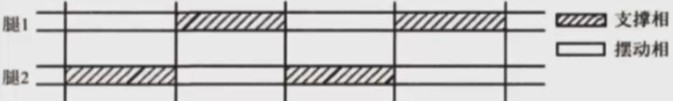
Timing diagram of walking and trotting
The first half cycle of the robot executes the support phase and the swing phase of the first half cycle according to the program, and adjusts the gait by recognizing the time increase on the basis of the set step frequency adjustment, and makes a state switch. In the same way in the second half cycle, the gait control of the robot can be realized.
Simulation Analysis
Kinematic Analysis
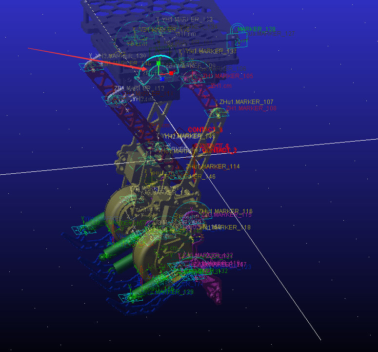
Based on the mechanical model established above for the robot leg mechanism, we perform dynamic simulation through ADAMS software, and draw the simulation results in the ADAMS post-processing module. The displacement and velocity simulation analysis is obtained. It can be seen from the figure that the robot’s running trajectory and running speed are relatively stable.
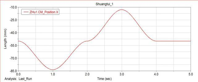
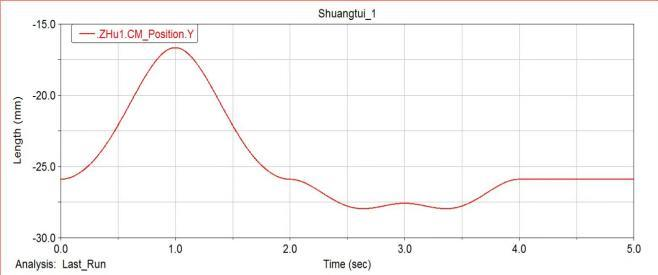
Simulation diagram of centroid displacement
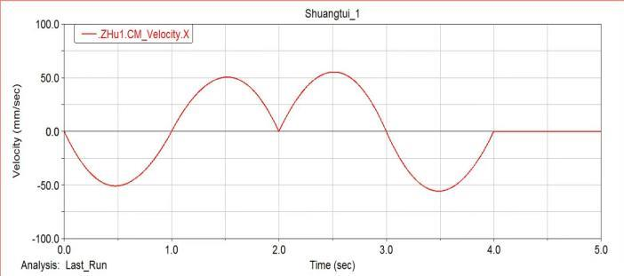
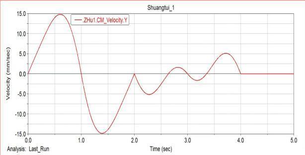
Center of mass velocity simulation diagram
Stress Analysis
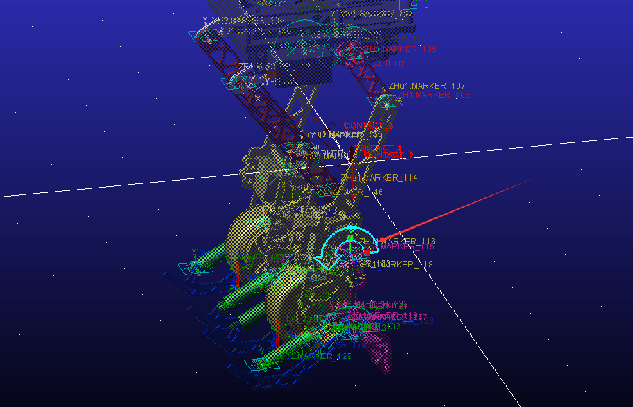
For the follow-up finite element analysis, based on the mechanical model established above for the robot leg mechanism, we perform dynamic simulation through ADAMS software, and draw the simulation results in the ADAMS post-processing module. The force of several dangerous places was obtained
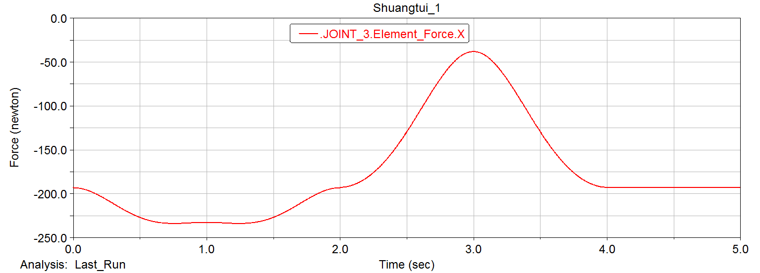
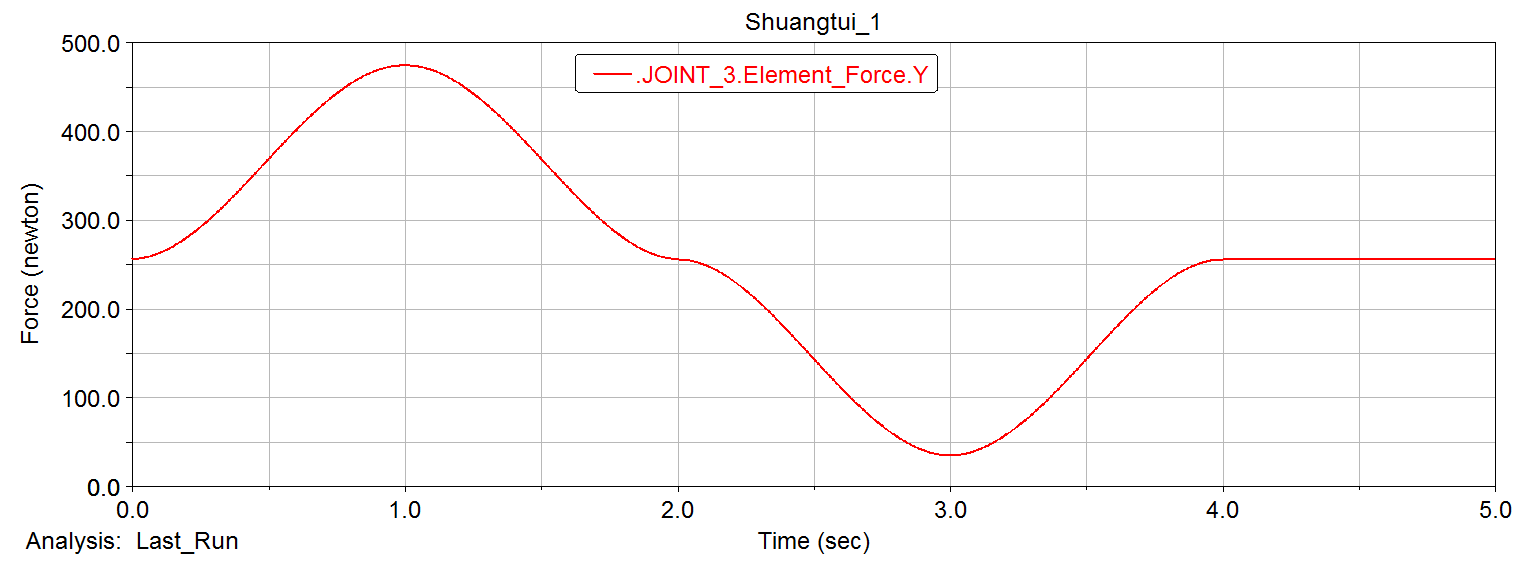
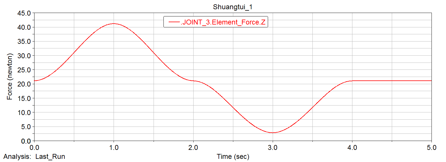
Three directions of force in xyz direction at the hinge of the main body and the leg structure
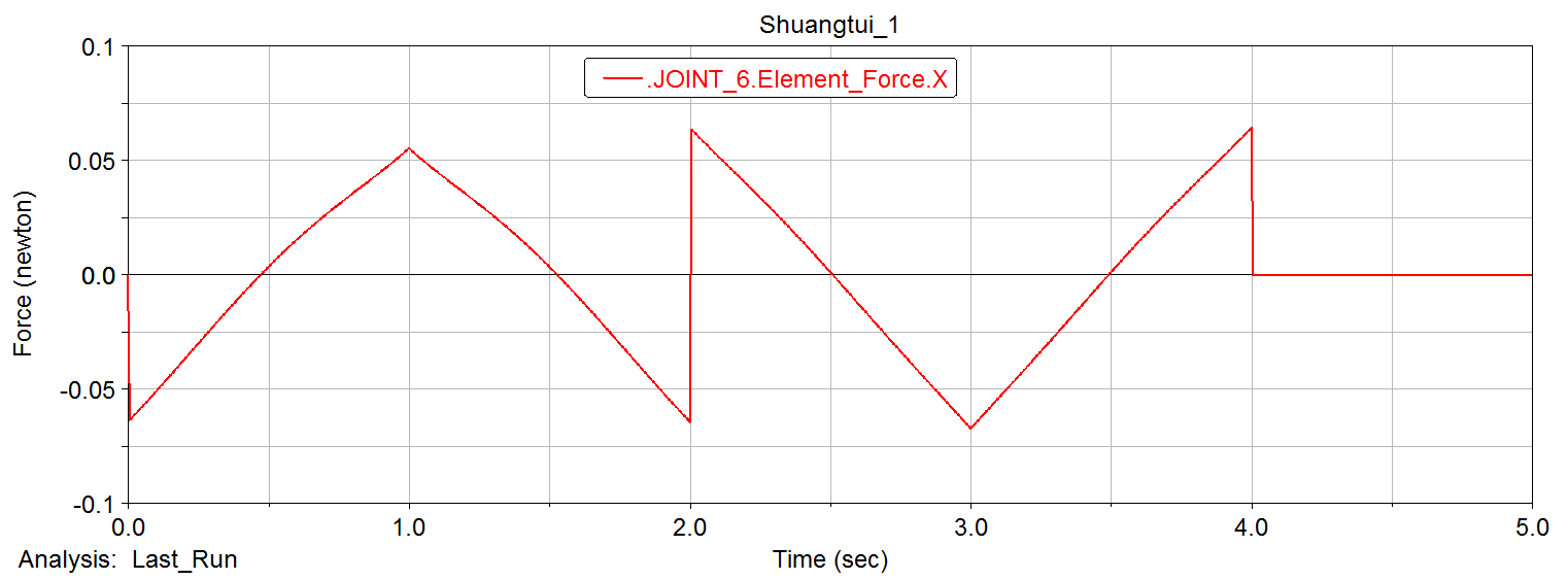
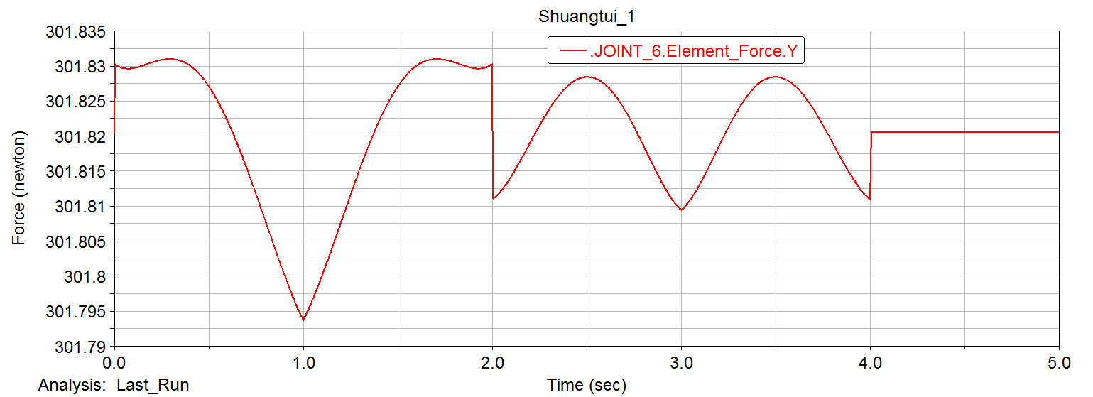
The force in the xy direction of the hinge of the leg and foot structure
Material and Process Selection
Material Selection
We initially selected the material as carbon fiber plate, and manufactured the parts through CNC process.
For general materials, the higher the specific strength, the better the performance under a given load. Metal materials such as aluminum are prone to problems such as deformation and dents under high loads, but carbon fiber composite materials are stronger under high loads because of their high specific stiffness and specific strength. Not only the performance advantages are obvious, but the highlight of carbon fiber composites is “lightness”, its density is only a little more than 1/2 of that of aluminum, which can provide more design space for power sources such as batteries. Longer battery life.
In addition, from an economic point of view, it seems that carbon fiber raw materials are much more expensive than aluminum alloys, but in specific applications, from raw materials to molding, the processing cost accounts for a larger proportion of the cost. However, through the efforts of many materialists, the price gap between carbon fiber manipulators and traditional aluminum alloy manipulators has been narrowed. At present, the price difference between the two is almost reduced to almost the same.
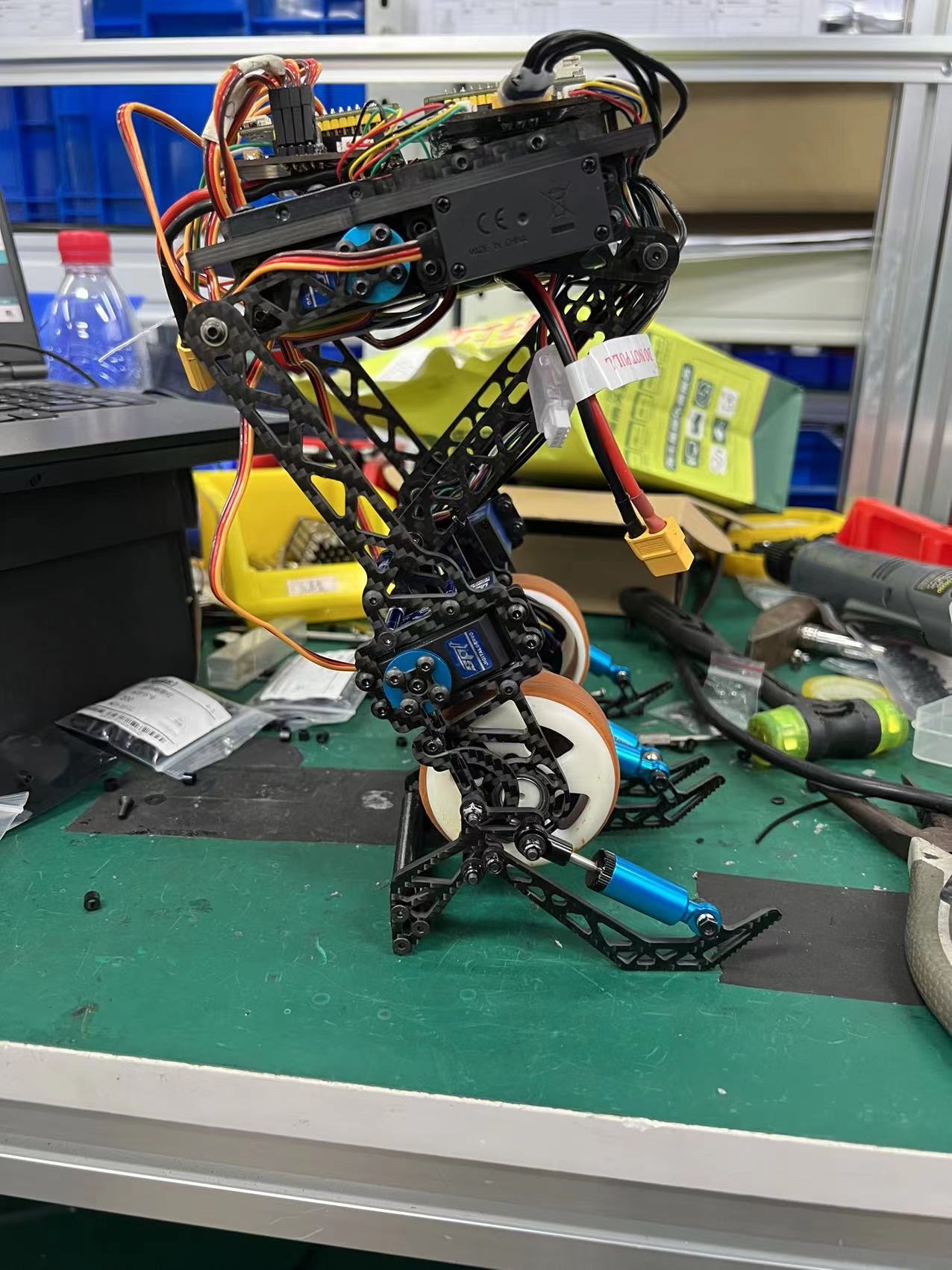
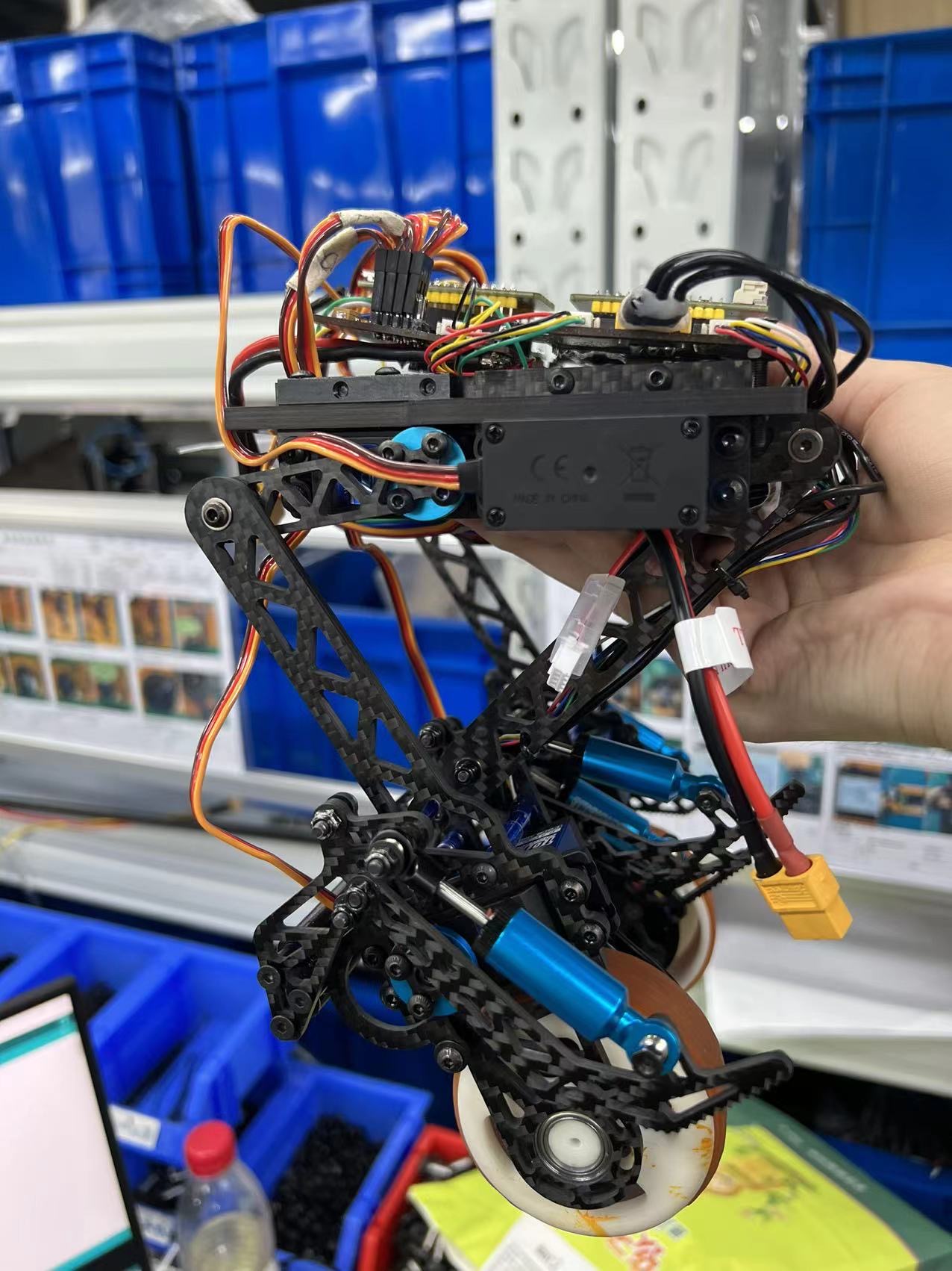
Robot assembled from carbon fiber parts
Strength Check
When the device is in the no-load state, the stress on each part is determined by the weight of the device itself, so the check of the dangerous rod focuses on the stress in the moving state. A dangerous condition is considered reached when the two rods that make up the main structure of the leg are folded close to horizontal. Now select two main rods composed of dangerous rods to make up the leg structure for finite element strength check. After adding loads as described above and performing adams simulation to obtain the force of each joint, use the Simulation module of SOLIDWORKS to perform finite element analysis, as shown in the figure below.
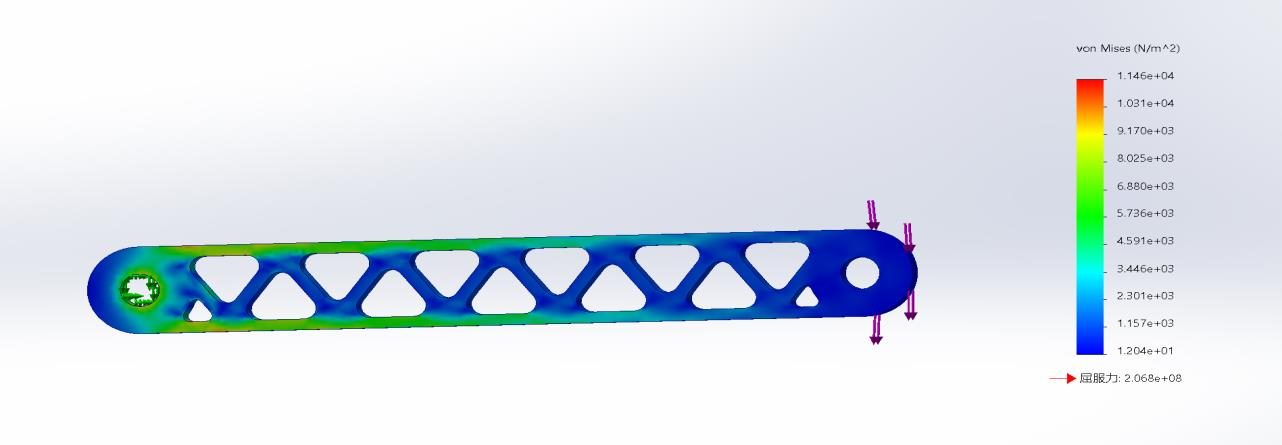
Finite element analysis of main rod 1
The calculated maximum stress is 11.46MPa. Carbon fiber is selected as the processing material, and the allowable stress meets the strength requirements by consulting the manual.
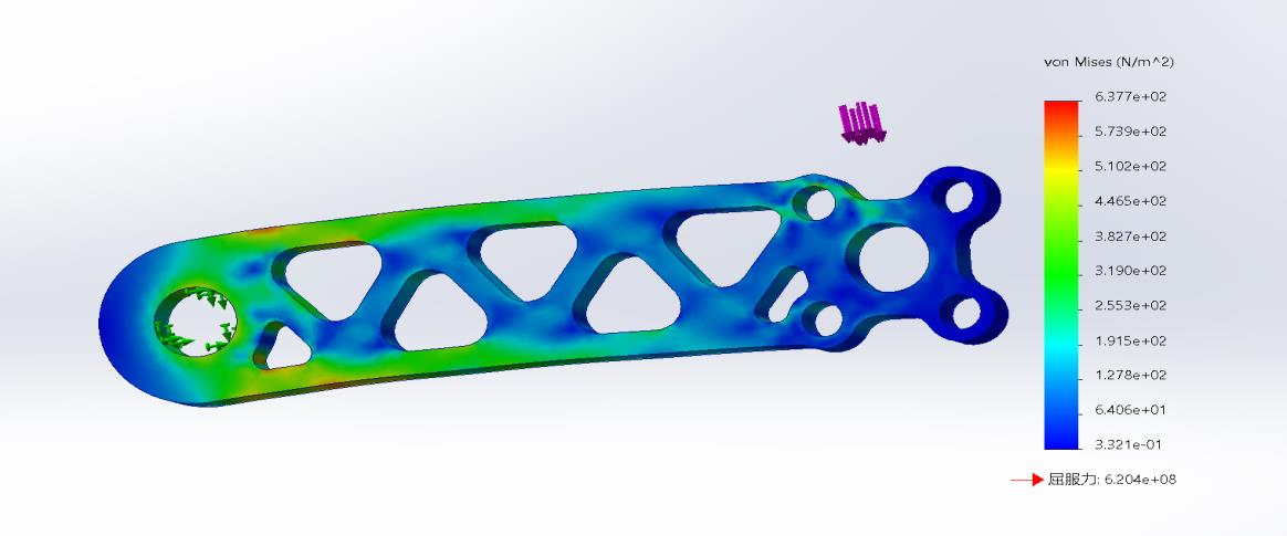
Finite element analysis of main rod 2
The calculated maximum stress is 0.6377MPa. Carbon fiber is selected as the processing material, and the allowable stress meets the strength requirements by consulting the manual.
Control System Design
Motor Parameter Calculation and Selection
Referring to the design of the bionic ostrich leg, after calculation, the motor voltage is 10v and the torque is 10N. After comparison, the motor is determined to be a brushless motor AS5048 encoder DC pod code disc micro-single motor zoom pan-tilt machine.
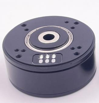
Brushless motor AS5048 encoder DC pod code disc micro-single motor zoom pan-tilt machine
| parameter | unit | 3510(magnetic ring) |
|---|---|---|
| Rated Voltage | V | 12 |
| Rated Current | A | 0.53 |
| Rated Torque | N*M | 0.11 |
| Rated Rotational Speed | rpm | 945 |
| Maximum Rotational Speed | rpm | 1250 |
Servo Parameter Calculation and Selection
After the force analysis according to the overall mechanical structure after 3D modeling, it is determined to add suitable materials and optimize the shape and size of the structural parts, and finally the weight of the entire mechanism is about AKG. Referring to the design of the legs of the bionic ostrich, it was determined that the servo was SPT5410HV-180/10kg high-voltage and high-speed digital servo.
Drivetrain Design
This device connects the motor to the calf construction and wheel-foot conversion on both sides, and connects the main components of the legs and feet in the form of multi-section levers, so as to drive the device to move back and forth as a whole. On the one hand, the motor at the calf drives the regular back and forth movement of the foot members on both sides, coupled with the adaptability of the foot components to the ground, and then drives the overall movement of the device. On the other hand, the motor at the wheel-foot conversion unit realizes the wheel-foot conversion by controlling the rotation degree of the hinge to rotate the wheel-foot adapter to the desired angle.
We directly bite the brushless motor and hub to form a direct drive structure. Higher precision and greater pressure resistance.
Drivetrain assembly drawing
Control Scheme Design
The control scheme of this device provides the offset angle for MPU6050, the servo realizes PWM control, and under the joint action of remote control, FOC drive board and magnetic encoder, it provides the control scheme of the whole device, and the whole control scheme is designed as follows:
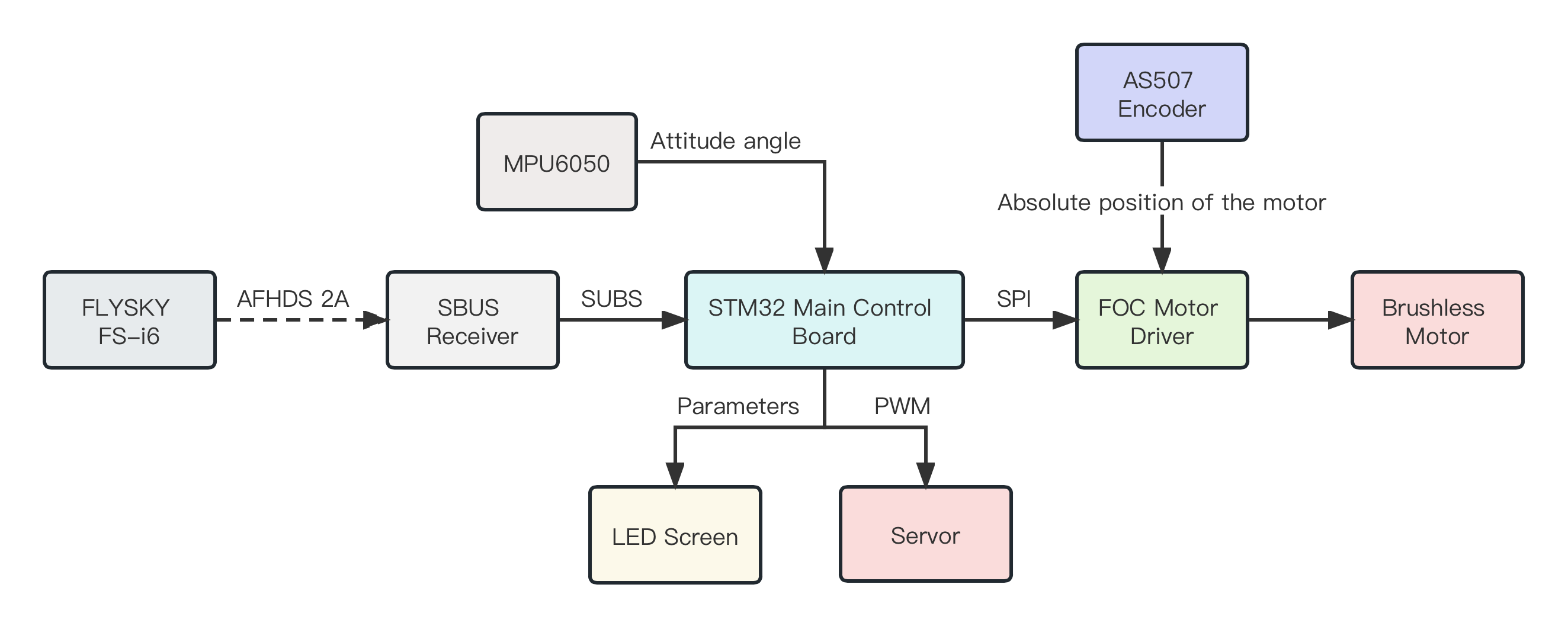
Control system diagram
Motor control design
PCB Design
The motor control drive system used in this device uses Esp32 as the main control, the ADC sampling rate is as high as 2M, and the FOC algorithm is used as the core control algorithm. As shown in the picture is the motor drive board.
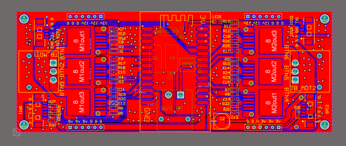
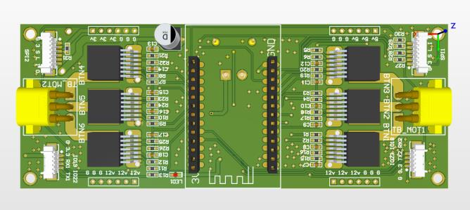
FOC driver PCB diagram
FOC Control Algorithm
Control at Low Speeds
Due to the difference in control principles, brushless ESC can only control the motor to work at high speed, and it is difficult to control at low speed; FOC controllers, on the other hand, do not have this limitation at all, and can be precisely controlled at any speed.
Motor Commutation
For the same reason, because the non-inductive ESC cannot feedback the rotor position, it is difficult to realize the commutation of the forward and reverse rotation of the motor; The commutation performance of the FOC driver is extremely excellent, and the forward and reverse switching can be very smooth at the highest speed; In addition, FOC can also perform brake control in the form of energy recovery.
Torque Control
Ordinary ESCs can only control the speed of the motor, while FOC can carry out three closed-loop control of current (torque), speed, and position.
Noises
The noise of the FOC driver will be much less than that of the ESC, because the ordinary ESC uses a square wave drive, while the FOC is a sine wave. Brushless The drive circuit of the motor is mainly realized by using a three-phase inverter circuit:
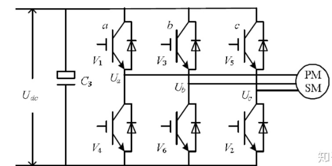
three-phase inverter circuit
Motor Parameter Acquisition
The idea of the LQR algorithm is adopted:
$$ \begin{aligned} J=q_{11} \theta^2+q_{22} \omega^2+q_{33} i^2+r U^2 \end{aligned} $$
Because $\theta$ is divergent, control as feedback is necessarily unstable, using $\Delta\theta$ as a feedback state variable. Since $\theta$ does not converge, the following equation is absolutely satisfied:
$$ \begin{aligned} & q_{11} \Delta \theta^2+q_{22} \omega^2+q_{33} i^2+r U^2 \leq q_{11} \theta^2+q_{22} \omega^2+q_{33} i^2+r U^2 \ \end{aligned} $$
$$ \begin{aligned} & q_{11} \Delta \theta^2+q_{22} \omega^2+q_{33} i^2+r U^2 \leq J . \end{aligned} $$
It can be seen from the above equation that $K_1$, $K_2$, and $K_3$ are the feedback coefficients of the state variables $\theta$, $w$, and $i$, respectively, so $K_1$, $K_2$, and $K_3$ must satisfy the state variables $\Delta\theta$, $w$, and $i$ for control.
Gait Control Design
It mainly adopts the algorithm of ZMP and linear inverted pendulum.
ZMP Algorithm
ZMP is the resultant force point of the ground against the robot calculated under the condition that the robot will not overturn, and when the robot is in dynamic motion (there is acceleration), the ground force is balanced with gravity and inertial force with ZMP as the action point. Since gravity does not change, when the height of the center of mass is unchanged, the position of ZMP (single point support, supporting polygon is a point) corresponds to the acceleration of the center of mass. The support point of the linear inverted pendulum is his ZMP.
ZMP algorithm
Linear Inverted Pendulum
The problem of linear secondary regulator (LQR) has a very important position in modern control theory and has received widespread attention from the control community. The linear quadratic performance index is easy to analyze, process and calculate, and the inverted pendulum system obtained by the linear quadratic optimal design method has the advantages of good robustness and dynamic characteristics and linear feedback structure, so it has been widely used in the actual design of inverted pendulum control system.
The input of the inverted pendulum system is the expected value of the displacement (i.e. position) of the bipedal robot and the tilt angle of the pendulum, and the computer collects the actual position signal of the robot and the reference surface from the sensor in each sampling cycle, compares it with the expected value, obtains the control amount through the control algorithm, and then drives the DC motor through digital-to-analog conversion to realize the real-time control of the inverted pendulum.
The principle of balancing a bipedal velocity ring:
According to experience, the running speed of the wheel-legged robot is related to the inclination angle of the wheel-legged robot, such as the wheel-legged robot leaning forward, is it the upright ring to accelerate the wheel-legged robot forward, so that the wheel-legged robot maintains balance, at this time the wheel-legged robot does not have speed. If the speed is controlled in a closed loop, then this loop is not a speed loop. If the target of the speed ring is set to 0, the wheel-legged robot can stabilize the balance for a long time.
However, in the balance car system, which is dominated by upright, the speed control of negative feedback will cause the trolley to accelerate down. Here we represent the control of the speed closed-loop by keeping the wheel leg robot at a certain angle and using the process of balancing the trolley.
Conclusion
Key Innovations
The innovation points of this device mainly include three innovative mechanisms and control algorithms:
Parallel five-pole structure
Since the tandem leg structure has high requirements for the joint drive motor and the control accuracy is difficult to guarantee, we use the closed-chain five-bar mechanism as the bionic leg structure, and the simulation results show that the leg structure can realize the rapid and stable running of the legs of the bionic ostrich, and the joint driving torque is small, which verifies the feasibility and rationality of the leg structure to realize the bionic gait running of the robot.
Wheel-leg composite structure
This bionic wheel-foot composite mobile robot combines the high efficiency of the wheeled robot on the flat road surface and the cross-country ability of the foot-type robot on the rough road, and the movement of the wheeled structure can cleverly mimic the ostrich whose toes are about to end the touch, so that the reaction force between it and the ground suddenly increases, resulting in the “pedaling force”.
Innovative variable foot mechanism
The wheel-foot mechanism switches freely through the two cells at the upper and lower dead center in the four stages of the entire trip, switching the movement mode, and a total of ankle joint, rigid grounded standing, electronic suspension, folding storage mechanical structure is ingenious.
Control algorithm
Adaptively adjusts left and right leg heights and controls body balance to cope with rapid movement on uneven ground. The LQR algorithm is used with the hub motor to flexibly and stably switch the robot motion state, such as the emergency stop movement during the running process.
Application Prospect
Wheel-legged composite robot is a new type of ground moving system based on wheeled robot by optimizing the wheel design to achieve fast and flexible movement. The main body of the robot is composed of a frame, two spindles, a gear reduction mechanism, and a wheel leg composite mechanism, which is driven by a single motor, and the control system is relatively simple. Compared with ordinary wheeled robots, the robot has a strong ability to cross obstacles, and has a lean structure, small size and light weight. This bionic wheel-foot composite mobile robot combines the high efficiency of wheeled robots on flat roads and the off-road ability of foot-based robots on rough roads, and has broad application scenarios.